In April 1902 Paul Rudolph, of the Carl Zeiss firm, applied for a patent for a camera or projection lens:

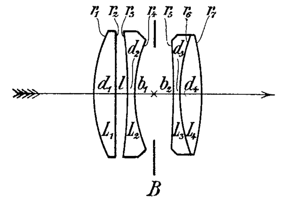
‘[Constructed by]… arranging four single lenses in two groups separated by the diaphragm, the two components of one of the groups inclosing an air-space between their two surfaces, facing one another, while the two components of the other group are joined in a cemented surface, and the pair of facing surfaces having a negative power…’

The full specification of the lens is included in the patent, but the wording is extremely broad. The Tessar is considered to be any lens of four elements, with a doublet and a pair of singlets. However, Rudolf Kingslake in The fundamentals of lens design gives more insight, describing them as like Protars but with an air-spaced front group, the Protar being another design from Rudolph and produced by Zeiss from 1890.

If we want to swap out those refractive index values for Abbe values we can simply fit Cauchy’s equation and use that to estimate the C-line index, giving the table below.

	nd (589.3nm)	Vd	∆P(g,f)
Lens 1	1.61132	58.4128	0.020117
Lens 2	1.60457	43.2243	0.012310
Lens 3	1.52110	51.5109	0.013207
Lens 4	1.61132	56.3675	0.021767

The original patent lists most of the values needed to model and construct the lens, however, you might struggle to find those particular glasses. A more modern formulation, from Kingslake, would find the same basic lens updated with modern (for 1978 in the case of my copy of lens design fundamentals) glasses, SK-3, LF-1, and KF-3, of note is the significant decrease in index of the second lens, but still flowing the same idea of a dense crown for the outer elements and medium flint for the second, and a light flint for the third.

The system focal length seems to be nominally 1000mm and back focal distance is 907mm. For the purposes of this exercise the presented designs will be scaled to exactly 1000mm focal length.

The lens produces an image circle of approximately 500mm. Requiring good performance over this size field is a challenge, but would be necessary if the camera was intended to be used without an enlarger. However, if only contact printing was intended then the definition requirement would be significantly lower. If the camera was to be used with wetplates then the chromatic aberration requirements become quite challenging, as the camera needs to be corrected for longitudinal chromatic aberration in the visible light (where it is focused) and the near-UV where most of the exposure comes from.

My initial hope/plan was to simply re-optimise this lens with modern computer optimisation and to get a slightly better performing lens at f/4 over the f/5.5 lens. This did not happen. It seems that Zeiss’s reputation was well earned. However, what I did do was significantly alter the lenses character and learn a lot on the way. For one, I didn’t really understand the importance of vignetting for aberration control, as you can clip off some of the problematic rays near the edge of the field of view, with only a small loss in edge illumination.

We can assess the performance of a photographic lens in a number of ways. From a design point of view one of the most obvious is spot size. This is the size that a single point of light would make at the focus of the lens. Different object distances can be considered, but for this I only looked at objects at infinity. Lenses tend to have better definition in the centre than at the edge, so it is important to examine the spot size at different field angles. Also, since lenses have dispersion it is important to also examine the effect of wavelength on the system. I used three main methods to judge image quality, the polychromatic spot size, chromatic focal shift, and image simulation. The image simulation also gives an idea of the performance of the whole system, including sharpness, chromatic aberration, and vignetting.

There are some things we do know about the lens such as properties of the glass and the radii of the curvatures. But there is also other information which we don’t know, such as the semi-diameters of the lenses, or the manufacturing tolerances of the system. If we guess at the first and ignore the second we can model the system as shown in the figures. The rear lens group is slightly smaller than the front group, vignetting some of the rays – this is set by the edge thickness of the rear lens.

To characterise this lens we might say that it is well optimised over the whole field, with the spot size increasing by more than a factor of 3 from the centre to the edge. The chromatic shift isn’t significant and at f/5.5 there isn’t any obvious lateral chromatic aberration.

I re-optimised the lens several times, tweaking the weightings of various factors. I decided that distortion wasn’t an issue, and that over-all central performance was more important the edge or the very centre. I also kept the same glass as the original. The prescription which I arrived at is

	Radii/mm		Thickness/mm
r1	213.366	L1	40.881
r2	-3276.842	gap	19.710
r3	-648.011	L2	11.081
r4	197.148	to stop	39.115
r5	-777.429	from stop	19.649
r6	221.080	L3	8.382
r7	-340.573	L4	46.140
		Backfocus	887.795

As can be seen from the table and the layout diagram the first lens of the re-optimised lens is almost unchanged. The second lens is slightly strengthened on both surfaces. The rear doublet is thickened and has more power. This might have been avoided in 1902 due to the cost of the ‘new achromat’ glass. Overall, the lens is not much changed, at least by examination. I expect that the 1902 patent lens would be less expensive to make due to the weaker surfaces and thinner lenses. However, in the re-optimisetion I did squeeze an extra stop of speed out of the system.

The re-optimised Tessar is a slightly better achromat with a smaller maximum chromatic focal shift of 766µm instead of the 916µm of the original Tessar. This is probably not significant. I don’t know exactly how the original lens was achromatised, however, my choice was to achromatise 0.54µm and 0.4861µm. These value were chosen as they are close to the peak sensitivity of the eye and of the collodion process, hopefully, a photographer could focus in the visible light and expose with minimal focus shift in the blue/near UV.

In the spot diagrams of the re-optimised lens you can see an obvious design choice, the centre spot has been allowed to increase in size slightly, and the very edge spot has increased significantly, all of the other regions show significant spot size decreases. This is due to a difference how I would personally like to compose images, with a less strong centre bias than 1902-Zeiss expected.

The average spot size for the re-optimised lens is significantly larger than for the patented example although almost all of that is in the very edge, but we can’t judge it too harshly as the re-optimised version is almost a stop faster at f/4 rather than f/5.5. If we stop it down to f/5.5 we get a slightly different result.

The spots have decreased significantly over the field when stopped down, as would be expected. The central spot size is now almost the same as in the patent design, and the 15˚ spot size is now smaller than the 7.5˚ spot size in the patent design – this significantly increases the region of good definition of the system.

Perhaps a more meaningful way of comparing the lenses is by simulating an image made from them.

Examining the simulated image (which doesn’t take into account depth) we can see some of the character of each lens. Like with any other artistic tool, the final judgement is based on the desired use.